Algebra

We will begin by going through a review of basic algebra. If seems too easy, feel free to skip to the next section; otherwise, continue here.

We will assume you know what negative numbers and fractions are, and how to do basic arithmetic. If not, review at https://www.khanacademy.org/math/pre-algebra.

The fundamentals of algebra¶

Algebra is a system of mathematics where we do computations using symbols rather than numbers. Symbols are usually denoted with roman or greek letters.

For instance, consider the following equation:

It’s clear that the “missing number” in the box has to be 8 for the equation to be true. We can now replace the box with a symbol called $x$:

Where:

The rules of algebra¶

Every unknown in algebra is denoted by a different symbol such as $x, y, z$, etc. For example, we could write:

Which would be true if $x = 1$ and $y = 2$.

Multiplication in algebra is written like this:

This means that:

And:

Division in algebra is almost always written as a fraction:

We can move the $x$ to the left of a fraction and it would be equivalent:

If we multiply a fraction by the same value as the bottom of the fraction, we get rid of the fraction:

If we have the same thing on the top and on the bottom of the fraction, we can remove the same thing - this is called “cancelling”:

The fraction of anything over one is itself:

We can move the bottom part of a fraction out of the fraction to get rid of the fraction:

We can have negative symbols as well as positive symbols:

A negative sign to the left of a fraction is equal to a negative numerator or a negative denominator:

Algebraic expressions are collections of numbers and symbols:

Equations are expressions that are related by an equal sign:

Parts of algebraic expressions and equations separated by operators ($+-\times \div$) or placed inside brackets are called terms. For example, $5x + 3y + 2z = 5$ has the terms $5x$, $3y$ and $2z$.

If we change the order of an equation, the equation remains the same:

Brackets are equivalent to multiplication when a number or symbol is placed to the left of a bracket:

We can expand brackets by multiplying the number (or symbol) in front of the bracket by everything inside the bracket:

And in the same way, we can factorize an expression into one that has brackets:

For more complicated brackets expansions, we use this formula:

To factorize this, we’ll need a tool called the quadratic formula, which we’ll explore later in this chapter.

We can write powers like this:

Where $x^3$ is equal to $x$ multiplied by $x$ 3 times.

Putting a negative sign in front of brackets is equal to multiplying everything inside the brackets by -1:

A double negative is a positive:

Sometimes, we use symbols to represent a number rather than an unknown - these are called constants. To avoid confusing symbols that represent numbers and symbols that represent unknowns, we usually use special letters (especially greek letters) to denote constants, and we will always say beforehand that the expression or equation contains a constant. For example, a common constant is $\pi$, which is a number that starts with the digits 3.14159. This means that:

Solving algebraic equations¶

To be able to solve algebraic equations, the key rule is that we do to the left-hand side of the equals sign as we do to the right.

For example, take the example:

Here, we first need to add $x$ to both sides of the equation, giving us:

This will become:

Which simplifies to:

We then subtract 5 from both sides of the equation:

And then divide both sides by 2 to get the answer:

Because $\frac{2}{2} = 1$:

Sometimes, we need to solve an equation that uses entirely symbols. Yes, that can seem scary, but going slowly, every step becomes easier. For example, presume we have the equation:

The first step is to multiply by $q^2$ on both sides:

Since we know that we can remove the $\times$ sign and just write symbols next to each other to show multiplication, this becomes:

We use one of the rules of algebra, which says that $\frac{a}{b} \times b = a$, to simplify:

This means our original equation becomes:

Now, we need to divide $p$ from both sides. Recall that we write divisions as fractions, so we have:

Using the rule that $\frac{px}{p} = x$, we can cancel the $p$:

Now, we can subtract $a$ from both sides to get rid of it:

Which gives:

We still unfortunately have the 2, which is more annoying to deal with. We have to divide the 2 from both sides:

Because $\frac{2x}{2} = x$ (it makes sense; multiplying something by a number then diving by that same number should give you that original something), we can simplify to:

Remember that anything multiplied by 1 is itself:

And that we can move parts of a fraction off the fraction:

Congratulations, we’ve solved it!

Graphs and coordinates¶

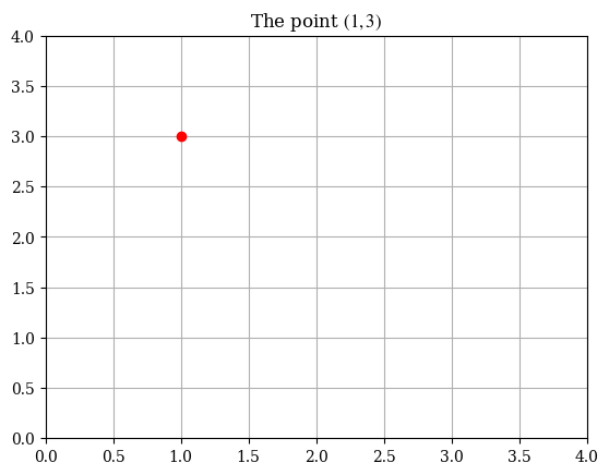
A graph is a visual way of representing data. To plot a graph, need two values: an $x$ value, and a $y$ value. We represent these values as ordered pairs like this:

For example, if we want to plot the value $x = 1, y = 3$, then $(x, y) = (1, 3)$. We can plot this on a graph by traveling 1 unit to the right, then 3 units up, like this:

import matplotlib.pyplot as plt
import numpy as np
# matplotlib-specific customizations
%matplotlib inline
plt.rcParams["font.family"] = "serif"
plt.rcParams['mathtext.fontset'] = 'stix'
plt.rcParams["axes.grid"] = True

plt.plot(1, 3, "ro")
plt.title("The point $(1, 3)$")
plt.xlim(0, 4)
plt.ylim(0, 4)
plt.show()

Functions¶

Functions take in a number and output another number. We denote a function with a symbol with the input as another symbol - for instance, a function $f$ with the input $x$ is written as $f(x)$. A simple function could be:

This means that any input $x$ value would have an output value of twice that $x$ value. We can make a table for values of this function:

We can visualize this table of values by plotting it as $(x, y)$ pairs, where $y = f(x)$:

x = np.linspace(0, 5)
plt.plot(x, 2 * x)
plt.title("$f(x) = 2x$")
plt.show()

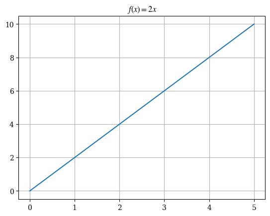
Since we plot the value of $f(x)$ on the y-axis, we say that $y = f(x)$. This means we could’ve called the above function $f(x) = 2x$, or $y = 2x$ - it doesn’t really matter.

Polynomial functions¶

Linear functions are in the form $f(x) = ax + b$, such as $f(x) = 5x$, where $a$ and $b$ can be equal to zero. They are called linear because they are “line-like” - they are straight lines. We’ve already seen this.

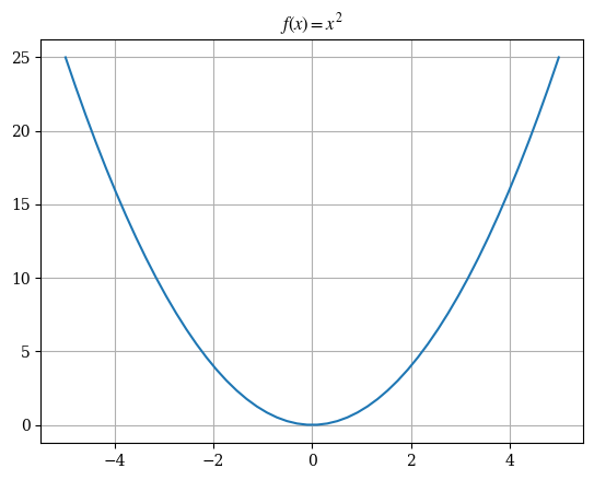
Quadratic functions are in the form $f(x) = ax^2 + bx + c$, such as $f(x) = x^2 + 2x + 3$, where $b$ and $c$ can be equal to 0. They look like this:

x = np.linspace(-5, 5)
plt.plot(x, x ** 2)
plt.title("$f(x) = x^2$")
plt.show()

We can solve any quadratic function in the form $ax^2 + bx + c = 0$ using the quadratic formula:

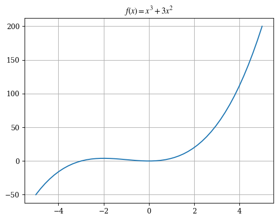
Cubic functions are similar, but they are just in the form $f(x) = ax^3 + bx^2 + cx + d$, such as $f(x) = 3x^3 + 5x^2 + 4x + 6$. They look like this:

x = np.linspace(-5, 5)
plt.plot(x, x ** 3 + 3 * x ** 2)
plt.title("$f(x) = x^3 + 3x^2$")
plt.show()

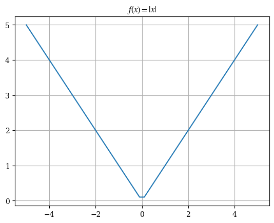
The absolute value function $f(x) = |x|$ takes in any negative or positive value and returns a positive value. It looks like this:

x = np.linspace(-5, 5)
plt.plot(x, np.abs(x))
plt.title("$f(x) = |x|$")
plt.show()

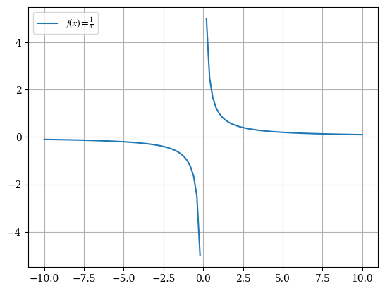
Rational functions¶

The rational function is in the form $f(x) = \frac{1}{x}$. It looks like this:

def f(x):
    with np.errstate(divide='ignore', invalid='ignore'):
        return 1/x
fx_name = r'$f(x)=\frac{1}{x}$'

x=np.linspace(-10,10,101)
y=f(x)
plt.plot(x, y, label=fx_name)
plt.legend(loc='upper left')
plt.show()

Trigonometry¶

Angles¶

An angle is the space between two lines that meet. We often represent angles using the symbol $\theta$, pronounced “theta”.

There are 2 main measurement systems we can use to define angles. The first measurement system is called degrees, denoted with the degree symbol °, where you can think of $360^\circ$ as one full circle. Thus, one angle of 1 degree is like slicing a circle into 360 pieces, and just taking one of those pieces.

The second measurement system is called radians, where one full circle is $2\pi$. This is a bit more abstract to understand, but you can use the same way to imagine: imagine taking a circle and cutting it into $2\pi$ (that’s around 6.283) pieces. What? Who would ever cut a circle into 6.283 pieces? Yes, it doesn’t make a lot of sense, but if you just think of one of those pieces, you would have an angle of 1 radian. We can convert between degrees and radians with:

Right-angled triangles¶

Trigonometry is the study of right-angled triangles - triangles that have one right angle and one other angle $\theta$.

The longest side of a right-angled triangle is called the hypotenuse. The opposite side is the the side that, well, is opposite the angle $\theta$. Finally, the adjacent side is the side between the right angle and the angle $\theta$.

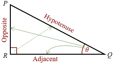
But wait, doesn’t a triangle have three angles? Yes, that is true, and so the choice of which angle you call $\theta$ doesn’t matter. You can define either one of the two other angles (the non-right-angle angles) as your $\theta$ angle, you just have to stick with one angle in your calculations.

Every right-angled triangle obeys the rule that:

Trigonometric functions¶

Trigonometric functions are oscillating functions that form a constant repeating pattern. The main, sine ($\sin$), cosine ($\cos$), and tangent ($\tan$), are defined by:

The reciprocal trigonometric functions are the normal trig functions but “flipped over”, and they look like this:

You can imagine taking a right-angled triangle and slowly making its angle $\theta$ bigger and bigger and bigger. The ratio between the sides is the value of the trigonometric functions.

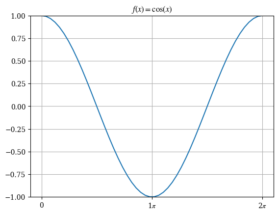
The graph of $f(\theta) = \sin(\theta)$, where $\theta$ is in units of radians, looks like this:

from matplotlib.ticker import FuncFormatter, MultipleLocator

f, ax = plt.subplots()
x = np.linspace(0, 2 * np.pi)
ax.plot(x, np.sin(x))
ax.set_ylim(-1, 1)
ax.grid(True)
ax.set_title(r"$f(x) = \sin(x)$")
ax.xaxis.set_major_formatter(FuncFormatter(
   lambda val, pos: f"{val/np.pi:.0g}" + r"$\pi$" if val !=0 else '0'
))
ax.xaxis.set_major_locator(MultipleLocator(base=np.pi))

plt.show()

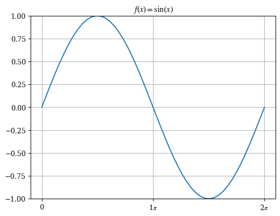
The values of $f(x) = \sin(x)$ can be deduced by reading off the graph:

Where $\pi \approx 3.14159$.

The graph of $f(x) = \cos x$ looks like the a shifted sine graph:

f, ax = plt.subplots()
x = np.linspace(0, 2 * np.pi)
ax.plot(x, np.cos(x))
ax.set_ylim(-1, 1)
ax.grid(True)
ax.set_title(r"$f(x) = \cos(x)$")
ax.xaxis.set_major_formatter(FuncFormatter(
   lambda val, pos: f'{val/np.pi:.0g}' + r"$\pi$" if val !=0 else '0'
))
ax.xaxis.set_major_locator(MultipleLocator(base=np.pi))

plt.show()

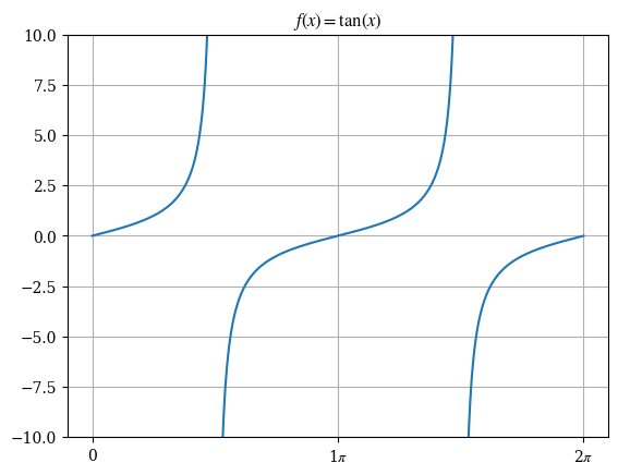
Whereas the graph of $f(x) = \tan x$ looks a little different:

def f_tan(x):
    with np.errstate(divide='ignore', invalid='ignore'):
        return np.tan(x)

f, ax = plt.subplots()
x = np.linspace(0, 2 * np.pi, 1000)
y = np.sin(x) / np.cos(x)
tol = 100
y[y > tol] = np.nan
y[y < -tol] = np.nan
ax.plot(x, y)
ax.grid(True)
ax.set_ylim(-10, 10)
ax.set_title(r"$f(x) = \tan(x)$")
ax.xaxis.set_major_formatter(FuncFormatter(
   lambda val, pos: f'{val/np.pi:.0g}' + r"$\pi$" if val !=0 else '0'
))
ax.xaxis.set_major_locator(MultipleLocator(base=np.pi))

plt.show()

Radicals¶

If we know a number, say, 4, can we find two equal numbers that multiply to form that number? Actually, we can! In the case of 4, we know that:

So we can say that the “square root” of 4 is 2, and we use the $\sqrt{}$ symbol to show this:

We can expand this idea. If we knew a number, say 8, can we find three equal numbers that multiply to form that number? Yes, we can! In the case of 8, we know that:

So we can say that the “cube root” of 8 is 2, and we use the $\sqrt[3]{}$ symbol to show this:

The same goes for 4 equal numbers that multiply to form a number, 5, 6, and so on. These roots, from the square root and cube root to that 4th and 5th and 6th root, are called radicals. Radicals follow these rules:

Exponentials and Logarithms¶

The rules of exponents¶

Exponents are every time we multiply one number by itself a certain number of times. For example, 2², pronounced “2 squared” or “2 to the power of 2” is two multiplied by itself, two times - that is $2 \times 2$. 2³, pronounced “2 cubed” or “2 to the power of 3” is two multiplied by itself, three times - that is $2 \times 2 \times 2$. Exponents follow these rules:

Fractional exponents are the same as a radical:

Finally, negative exponents are equal to one over the positive exponent of that number:

Exponential and logarithmic functions¶

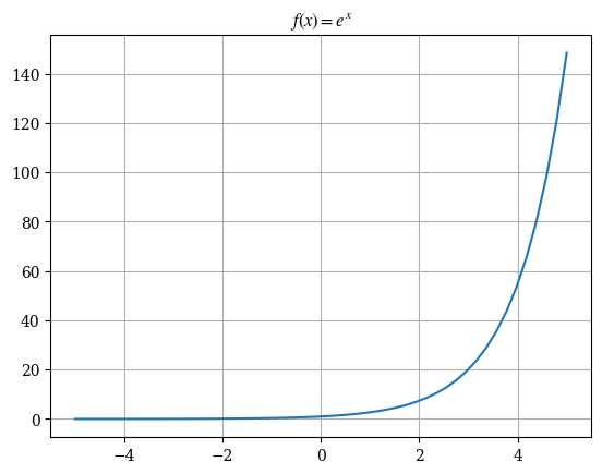
All exponential functions are in the form $f(x) = b^x$ where $b > 0$ and $b \neq 1$. Note that if $x$ is negative, then $b^{-x} = \left(\frac{1}{b}\right)^x$. The most commonly-used exponential function is $f(x) = e^x$, also confusingly called “the exponential function”, where $e$ is a special number that is around 2.718:

x = np.linspace(-5, 5)
plt.grid(True)
plt.plot(x, np.exp(x))
plt.title(r"$f(x) = e^x$")
plt.show()

What if we want to “undo” the exponential function? We would need to find an inverse function, a function that does the opposite thing as another function. In the case of an exponential function, the inverse is called a logarithmic function. The basic logarithmic function is given by:

where $b^y = x$. To remember this mapping between exponential functions, you can remember that $b$ is the “basement” (because of its subscript), and it’s raised to the “answer” of $y$ to get $x$. Several common logarithmic functions have shorthand notations:

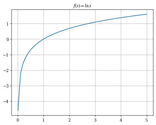
The $\ln$ function is also called the “natural logarithm”, and it looks like this:

x = np.linspace(0.01, 5)
plt.grid(True)
plt.plot(x, np.log(x))
plt.title(r"$f(x) = \ln x$")
plt.show()

Just as with exponents, logarithms follow certain rules:

Factorials¶

A factorial is when you multiply a number by all whole numbers smaller than it, and is denoted with $!$. For example, $2! = 2 \times 1$, $3! = 3 \times 2 \times 1$, and $4! = 4 \times 3 \times 2 \times 1$.

Sums¶

Sometimes, we want to add up a lot of numbers:

How do we compactly write this out? One way is to assign each number a symbol, with its position in the list of numbers to add as an index on the bottom. So 1, which is the first number, would be $a_1$. This becomes:

A compact way of writing this out is with the summation symbol:

where $i$ is the index on the bottom, $i = 1$ means the indices start from 1, and $n$ means the indices end at $n$. $n$ can be infinity sometimes:

Summation is very useful for shortening long formulas. For example, the binomial expansion formula: