Differential equations

“Science is a differential equation. Religion is a boundary condition.”

Alan Turing

Differential equations are simultaneously often regarded as some of the coolest and strangest objects in physics. On one hand, they’re ubiquitous, and nearly every physics theory is expressed using them. On the other, they have a tendency to be unsolvable and difficult to understand. It is hoped that this chapter will bring all their positive qualities into the limelight, and make differential equations no longer scary or intimidating, but descriptions of nature unrivaled in their beauty.

What is a differential equation?¶

Differential equations are any equations that describe a function in terms of how it changes through space or time. For instance, we could have:

The interpretation of this equation is that $y$ increases proportional to its derivative, so as $y$ increases, the rate of change of $y$ increases by a proportional amount.

Differential equations can be of a single-variable function and its derivatives, or a multivariable function and its partial derivatives. For instance, the wave equation is given by:

Here, $u = u(x, t)$, and is the function describing the wave. The interpretation of the wave equation is that the rate of change of the rate of change of $u$ moving along the $x$ direction is proportional to the rate of change of the rate of change of $u$ as time passes.

Differential equations that only involve single-variable functions are called ordinary differential equations (ODEs), while those that involve multivariable functions (and their partial derivatives) are called partial differential equation (PDEs).

Initial-value and boundary-value problems¶

We are interested in solving differential equations to be able to perform further mathematical analysis of the physics of a given system. There are a myriad number of ways to solve differential equations, and we will cover just a few in the following sections. In general, however, finding an exact solution to a particular system cannot be done with knowledge of just the differential equation; typically, some data must be provided before a solution can be found.

In the case of ODEs in the form $\dfrac{dy}{dt} = f(t, y)$, this data is called the initial condition, the state of $y(t)$ at $t = 0$. Some physical examples of initial conditions are the initial velocity or initial position. We often denote such an initial condition $y_0$. Once we know that, we can calculate the values of $y$ that the differential equation predicts for all future times $t$. The combination of an ODE and an initial value is known as an initial-value problem (IVP).

Boundary-value problems can be thought of as an extension of initial value problems to partial differential equations (PDEs). Unlike initial counditions, boundary value problems usually specify the function that the solution to the PDE takes at the boundaries. Such functions are called boundary conditions (BCs). A physical example may be some water sloshing in a water tank; a PDE may be solved to find the function describing the distribution of water within the tank. The boundary condition would then be the height of the water at the walls of the tank.

The three main types of boundary conditions are Dirichlet, Neumann, and Robin. You can mix and use different boundary conditions together, especially for boundary-value problems that have different types of boundaries, but individually they are generally in one of these forms:

Physical significance of different types of boundary conditions¶

The physical intepretation of a Dirichlet boundary condition is that the physical quantity is fixed or constrained at the boundary, that is, it takes a specific constant value. In the special case where $u = 0$ at the boundary, the physical quantity vanishes at the boundary.

Meanwhile, the physical interpretation of a Neumann boundary condition is that the physical quantity is kept within the boundary. This corresponds to insulating or reflecting boundaries that prevent the physical quantity from flowing or radiating outwards.

Robin boundary conditions have more flexible physical interpretations. One specific type of robin boundaries is an open boundary. The physical interpretation of an open boundary condition is that the physical quantity is allowed to flow undisturbed outwards beyond the boundary. This corresponds to boundaries that allow for outward radiation or free propagation through them. It is a specific type of Robin boundary condition.

Solving initial- and boundary-value problems¶

Initial-value problems can be solved by hand in some cases, but for cases where they cannot be solved by hand, computational methods can be used to solve them numerically (this results in an approximate solution). We will explore how to do so in the numerical methods section in Chapter 3. In addition, there exist online calculators that numerically solve differential equations: see Bluffton University’s free tool at this link for solving IVPs.

Boundary-value problems can be solved by hand in vastly fewer cases, and even when a solution is possible to find by hand, many simplifying assumptions must be used. For this reason, numerical methods are required for the majority of boundary-value problems. Again, we will explore this further in Chapter 3, but for those interested, the web app Visual PDE provides an easy-to-use graphical interface for solving PDEs numerically. We recommend you try it out!

Solving differential equations¶

When we are told to solve a differential equation, what we are doing is to figure out $y$ from the differential equation. How we can do this depends on the type of differential equation. For example, consider an ODE in the form:

If we can put any ODE in this form, it is considered separable. What we can then do is to make sure each side of an equation is expressed only in terms of one variable:

And finally, to integrate both sides to solve:

Partial differential equations are considered separable by a similar criteria: if you can express each side of them only in terms of one variable, then they are separable.

But enough theory! Let’s actually try solving two differential equations, one ODE and one PDE. The ODE we will be solving is the exponential growth equation - the reason for that name will become apparent very soon. It is given by:

Here, $k$ is just a constant. To solve for $y$, we must isolate each side to single variable. To do so, multiply each side by $dx$, so

Then, divide both sides by $y$ to get

We can now integrate both sides to solve:

Which results in:

We raise both with $e^x$, to get:

Which becomes:

Just one more step! Now that:

If we define a new constant $C_2 = e^C$, then:

This is called the general solution to the exponential growth equation, because $C_2$ can be any number, and so this general solution encodes all possible solutions each with their own value of $C_2$.

To actually solve it for a value, we need an initial value. For instance, we may be told that $y(0) = 1$. If we plug that in:

So our unique solution given our initial value is now:

We have now solved the initial value problem - finding the solution to the differential equation given the provided initial condition.

Note that $C_2$ was the same number as $y(0)$. Therefore, we have a new interpretation of $C_2$ - note that $C_2$ is the initial value of a function, so $C_2 = y_0$, and we can rewrite the general solution as:

The PDE we will be solving is the 1D heat equation, given by:

where $k$ and $L$ are constants. This equation models the temperature function $u(x, t)$ of a long, thin rod, where the value of $u$ at a given position $x$ and a given time $t$ is the temperature. Third nice fact about the equation: it’s separable! To separate, we first write $u(x, t)$ as a product of two functions:

Therefore, using this definition, we can compute the partial derivatives of $u$:

So we now have:

This also applies applies to the boundary conditions as

These equations imply that one of two cofficients in each equation must be zero. Because the trivial solution is unacceptable, the function $f(x)$ can not be equal to zero. Therefore, the new boundary conditions become

Going back to the new formation of the PDE using the separated functions, it can be rearranged into

This isolates the left side to functions of $t$ and the right side to functions of $x$. Therefore, one variable changed, its side will change while the other would stay the same. Therefore, because this will violate their equality, both sides must the same. Therefore, they are both equal to a constant, $-\lambda$:

Why the negative sign? Since a negative sign applied to a constant makes it still a constant, so we can technically do what we want to $\lambda$ - scale it, add another constant to it, make it positive or negative, the math still works out. The only difference is that $-\lambda$ makes the resulting differential equations way easier to solve because $\lambda$ will be positive once the new ODE is formed.

The introduction of the constant allows us to separate the PDE into two ODEs that easier to solve:

For the first equation,

The first equation is a linear, second-order, homogeneous, constant-coefficient equation. Therefore, the solution is in the form $f(x) = e^{rx}$ where $r$ is an unknown constant. Then, by substituting this into the equation,

Because $\lambda$ is unknown and the solution is dependent on its sign, consider the three case $\lambda > 0$, $\lambda <0$, and $\lambda = 0$. If $\lambda > 0$, then let $p^2 = \lambda$ where $p > 0$. Then,

Therefore, the solution becomes

Using Euler’s formula, the equation becomes

where $C= A+B$ and $D=(A-B)i$. Implimenting the first boundary condition $f(0) = 0$,

This transforms the equation into

Implimenting the second boundary condition $f(L) = 0$,

$D$ can not be zero because it will result in $f(x) = 0$, so $\sin(pL) = 0$. Using trigonometry, the equation becomes

where $n=1, 2, 3 , \ldots$. Therefore, in the case if $\lambda > 0$,

In the next case where $\lambda < 0$, let $\lambda = -p^2$ where $p > 0$. Then,

Therefore, the solution has the form

Implementing the first boundary condition $f(0)=0$,

Therefore,

Implementing the second boundary condition $f(L)=0$,

Because $p > 0$ and $L \ne 0$, this statement is invalid. Therefore, the second boundary condition isn’t satisifed and the case can not exist. Then, moving to the third case $\lambda = 0$, so $r=0$. Therefore,

Using both boundary conditions, $f(x) = 0$. However, because this solution is the trivial solution, it is also invalid. Therefore, this case can not exist, thereby leaving the only valid case to be where $\lambda < 0$. Therefore,

where $\lambda = \frac{n \pi}{L}$. Now, going back to the second equation from the original, $g(t)$ is calculated as so

where $C$ is an unknown constant of integration. Then, using the seperablility of $u(x,t)$, it can calculated with product of the two solutions as so

Because $n = 1,2,\ldots$, there infinite number of solutions to the heat equation. Therefore, using the linearity of the equation, all the solutions can be combined into an infitie sum will form the ultimate solution of the equation as

To solve for the unknown constant $C$, we will impliment the initial condition $u(x,0) = f(x)$ to solution to get

Because the sine function is orthogonal to itself, $\int \sin(\frac{n \pi x}{L}) \sin(\frac{m \pi x}{L})dx = 0$ with an integer $m$ if $m \ne n$. Otherwise, $\int \sin(\frac{n \pi x}{L}) \sin(\frac{m \pi x}{L}) dx = \frac{L}{2}$. Using this information, we can multiply both sides of the equation by $\sin({m \pi x}{L})$ and integrate both sides with respect to $x$ to eliminate the infinite number of sine functions. Once done, the equation reduces to

Because $m$ equals the $n$ in which the only constant is under, $m$ be replaced with $n$ in this equation and can rewritten to the solution

Therefore, the 1D heat equation is solved.

Laplace Transform¶

Suppose you must solve for $y(t)$ for the inhomogeneous, initial value problem

with some known initial conditions. There are several ways to solve this problem, but one of them is through Laplace Transformations. To define this, suppose $f(t)$ is a piecewise smooth, continuous function on $0<t< \infty$ such that $|f(t)| < Ce^{kt}$ for some $C>0$ and $k \ge 0$, which bounds $f(t)$ by exponential growth. Therefore, the Laplace Transformation of $f(t)$ is defined as

This solves the equation before by taking the Laplace Transformations from each side, solving the Laplace transformation of $y(t)$, noted as $Y(s)$, and taking the inverse Laplace transformation of both sides to solve for $y(t)$. To do the former, because of the repeatability of the technique, there are many repeatable transformations listed as such:

In the case of derivatives,

Therefore,

Furthermore, Laplace transformations has both properties of linearity and translation, respectively meaning

where $c_1$, $c_2$ are arbitrary constants.

To demonstrate, suppose

To solve for the Laplace transform of $y(t)$, $Y(s)$, for this problem, we must apply the Laplace transformation to both sides of the equation

Then, we must translate each side of the equation. For the left side,

For the right side,

Therefore,

To reverse the translated equation back to its original properties, an inverse Laplace transformation must be used. The inverse Laplace transform is defined such that $\mathcal{L}^{-1} \{F(s)\} = f(t)$ whenever $\mathcal{L} \{f(t)\} = F(s)$. The inverse Laplace transform retains the properties of linearity and transformation respectively as

as well as reverse the operations displayed in the table previously.

However, the perform the inverse Laplace transformation on the pervious equation, it must be expanded using Partial Fraction Decomposition. Suppose $\frac{P(s)}{Q(s)}$ such that $\deg P < \deg Q$. If $Q(s) = c(s-s_1)(s-s_2) \ldots (s-s_n)$, then

where $A_i = \lim_{s \to s_i} (s-s_i) \frac{P(s)}{Q(s)} = \frac{P(s_i)}{Q'(s_i)}$ for all $i = 1,2,\ldots, n$.

If $Q(s) = c(s-s_1)^{n_1} (s-s_2)^{n_2} \ldots$ where $c$ is an arbitrary constant, then

If $Q(s) = c((s- \alpha_1)^2 + \beta_1^2)((s-\alpha_2)^2 + \beta_2^2)\ldots$, then

Revisiting the original problem,

Using Partial Fraction Decomposition,

Multiplying each term on the right hand side such that the denominator of each term matches the denominator of the left hand side,

For the limit $\lim_{s \to 2}$,

Therefore,

For the limit $\lim_{s \to 3}$,

Therefore,

For the limit $\lim_{s \to 1}$,

Therefore,

For the limit $\lim_{s \to 0}$,

Therefore,

Substituting into the resulting equation from $\lim_{s \to 1}$,

For the limit $\lim_{s \to 4}$,

Therefore,

Using the same substitution of $A_3$,

Therefore,

Therefore,

Therefore,

Using the inverse Laplace transformation on each side,

This completes the problem and the section.

Fourier Series¶

Let $f(x)$ be defined for $-L < x< L$. The Fourier series of $f(x)$, $F(x)$, is given by

It is found in the solutions of many PDEs including the heat equation, Laplace’s equation, and the wave equation, and its coefficients can be solved using the orthogonality of sine and cosine and are

An important property of a function of a Fourier Series is piecewise smoothness. To explain, let $f(x)$ be defined for $x \in [a,b]$. The function is piecewise smooth if a finite partition of $[a,b]$ exists such that $f(x)$ and $f'(x)$ are continuous on each sub-interval of the partition and that one-sided limits exist at the boundaries of the sub-intervals.

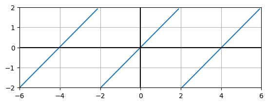
This is important because this quality allows the Fourier Series to converge into a periodic extension. If $f(x)$ is piecewise smooth, then the periodic extension of $f(x)$ is the periodic repetition of $f(x)$. For example, if $f(x) = x$ along $-L<x<L$, then its periodic extension forms

import matplotlib.pyplot as plt
import numpy as np

L = 2
N = 3 # number of periods to display
samples_onethird = 50 # number of samples / 3
x = np.linspace(-N*L, N*L, samples_onethird*N)
x_original = np.linspace(-L, L, samples_onethird)
x_original[-1] = np.nan
y = np.tile(x_original, N)

plt.plot(x, y)
plt.grid()
plt.gca().set_aspect("equal")
plt.axhline(y=0, color='k')
plt.axvline(x=0, color='k')
plt.ylim(-2, 2)
plt.xlim(-N*L, N*L)
plt.show()

The Fourier Convergence Theorem states that if $f(x)$ is piecewise smooth along $-L<x<L$, the Fourier series of $f(x)$ converges to the periodic extension of $f(x)$ where $f(x)$ is continuous and the mid-point of the one-side limits at each jump discontinuity. This allows us to graph the function of Fourier Series and, by extension, the solution of most PDEs.

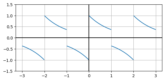
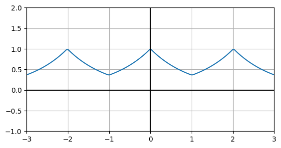
If one of the coefficients of the summations in the original Fourier Series $F(x)$ were equal to zero, then the series would reduce into a half-range series and the graph of the function changes. If the summation with coefficients of sine functions remains, then the Fourier Series transforms into a Fourier Sine Series and an odd function, which means $f(-x)=-f(x)$. 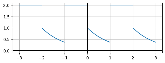On the other hand, if the summation with coefficients of cosine functions, then the Fourier Series transforms into transforms into a Fourier Cosine Series and an even function, which mean $f(-x) = f(x)$. To demonstrate this change, let

where $f(x)$ is a piecewise function for $1<x<-1$. The Fourier Series of $f(x)$ converges to

# The function is y=2 x<0, y=e^{-x} x>0
eps = 0.01
L = 1
N = 3 # number of periods to display
samples_onethird = 200 # number of samples / 3
x = np.linspace(-N*L, N*L, samples_onethird*N)
x_original = np.linspace(-L, L, samples_onethird)
y_original = np.piecewise(x_original, [x_original< -eps, abs(x_original) <= eps, x_original>eps], [lambda x: 2, np.nan, lambda x: np.exp(-x)])

# Force breaks in curve via NaNs
y_original[-1] = np.nan
y_original[0] = np.nan
y = np.tile(y_original, N)

plt.plot(x, y)
plt.grid()
plt.gca().set_aspect("equal")
plt.axhline(y=0, color='k')
plt.axvline(x=0, color='k')
plt.show()