Electrodynamics
“We can scarcely avoid the inference that light consists in the transverse undulations of the same medium which is the cause of electric and magnetic phenomena.”
James Clerk Maxwell
In the first chapter, we introduced the classical theory of electricity and magnetism. We discussed electric and magnetic fields, and we ended with a discussion on Maxwell’s equations and electrodynamics. Now, we will take a closer look at electrodynamics - and gain critical insights into the nature of light and the electromagnetic field.
Formulations of the Maxwell equations
We will start by reviewing the Maxwell’s equations. Written in the language of vector calculus, they take the form of a system of four partial differential equations, which we show below:
This form is excellent for conceptual understanding and for illustrating the relationships between the electric and magnetic fields. However, it is rather poorly-suited for actually finding solutions. First, there are four PDEs to solve, and second, the last two PDEs are coupled, meaning that they cannot be solved independently of each other.
But we can simplify the Maxwell equations into a more tractable form. First, we can reduce the number of equations to solve, because, technically, the first two equations are just constraint equations. That is to say, these two equations don’t need to be solved because they are implicitly satisfied for any solution of Maxwell equation #3 and Maxwell equation #4, a result first derived by J. A. Stratton in 1941. To show this, let’s first take the divergence of the time derivative of . We get:
Where we substitute in the left-hand side of Maxwell equation #3 and use the vector calculus identity that the divergence of the curl is always zero (the vector calculus identities Wikipedia page is a highly-useful resource when doing a lot of vector calculus). But remember, taking the divergence only affects the spatial components of fields (because , there is no time-dependent part in it) so we can swap the time derivative operator and the divergence operator:
However, we already found that , so:
This means if the initial condition for the magnetic field obeys , then holds for all times , and therefore, Gauss’s law for magnetism is automatically satisfied for any solution of just the last two of Maxwell’s equations.
Meanwhile, we can rearrange Maxwell equation #4 to have the time-derivative on the left via:
Which, knowing that , we can simplify to:
Taking the divergence of both sides, we get:
Again, due to the fact that taking the divergence doesn’t include taking any time derivatives, we can swap out the time derivative and divergence operators, that is:
So substituting that in, we have:
But due to charge conservation, the current density and charge density are related by the partial differential equation:
This is the continuity equation for charge conservation and it means that charge can never be created or destroyed, just moved around. If we rearrange it, we get:
If we substitute this into which we derived two steps before, we get:
So that we have the relation:
Rearranging the terms and doing some straightforward rewriting, we get:
But we know that is just a different way of writing Maxwell equation #1, which is Gauss’s law for electricity! So if the initial condition for the electric field obeys , then holds for all times , and therefore, Gauss’s law for electricity, just like Gauss’s law for magnetism that we looked at earlier, is also automatically satisfied for any solution of just the last two of Maxwell’s equations. To our relief, this means that so long as we check our initial conditions to ensure that the divergence of both the electric and magnetic fields is zero, Maxwell’s equations reduce to just two coupled PDEs!
In free space, that is, when we’re not considering any current sources, we can set , meaning that as well as . Maxwell’s equations then become:
If we take the curl of both sides of each, we find that:
Using the double-curl vector calculus identity , and swapping the time derivative and curl operators (remember that like the divergence, the curl is spatial-only, doesn’t have any effect on time), we have:
But we know what and are from Maxwell equations #3 and #4, and we can substitute those in:
Equating these expressions with the expressions we got by applying the double-curl identity, we get the wave equations that we analyzed earlier:
So we can summarize the results as follows:
| Configuration | System of equations | Interpretation |
|---|---|---|
| Free space (no current/charge sources) | EM waves | |
| General case (can have current/charge sources) | Any EM field configuration |
But again, the PDEs themselves are not enough. For a complete boundary-value problem, we also need the boundary conditions, and those come from the physics we want to model. We will now look at different boundary-value problems in which we can solve the Maxwell equations analytically.
Solutions to the electromagnetic wave equation
The solutions to the first case - the Maxwell equations in free space - are of particular interest, as their solutions describe electromagnetic waves. The first, and simplest, solution that we will examine is that of the plane wave, given by:
Which is sometimes written in more compact notation as:
Where is the wavevector and is the angular frequency of the wave, and is the phase shift (which we can set to zero). Note that plane waves describe vector-valued electric and magnetic fields, so is a vector. This vector is the product of the field amplitude and , the polarization vector, defined as follows:
Or written in equivalent complex exponential form (recall: ), omitting the phase shift for now since we can always include it back in later:
The magnitude (electric field strength) is then given by:
Where is the normal vector that points in the direction of propagation of the wave. Of course, complex-valued waves are just for mathematical convenience; to get any physically meaningful results, we only consider the real part of the complex exponential, and ignore the imaginary part.
Recall that the output of the function is the magnitude of the wave, and in electrodynamics it is associated with the magnitude of the electromagnetic field at that point. In 1 dimension, this is the familiar sinusoidal wave; in 2 dimensions, this becomes a sinusoidally-rippling surface, see https://
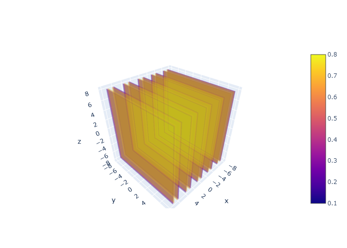
The magnitude of the electric field for a plane wave, which oscillates sinusoidally along the direction of propagation.
The intensity still varies sinusoidally, but the wavefronts are planar, as is expected. Note that plane waves are a mathematical idealization; true waves are only approximately planar and would spread out over long enough distances.
We now want to find the associated field from the electric field. To do so recall the third of Maxwell’s equations:
Taking the curl of is highly nontrivial; however, luckily, we have a very nice identity that where . Be aware that , the unit vector of the electric field is not the same thing as the normal vector in the argument of the complex exponential! The electric field has , remember the unit vector doesn’t care about magnitude, only direction, so these two are equivalent. The in the argument of the complex exponential is the direction of propagation of the wave, but is the unit vector, i.e. the direction that the electric field is aligned. These are not the same thing because electromagnetic fields are transverse; the electric field oscillates up and down, but the wave moves forward.
With that distinction out of the way, we can resume the calculations. The magnitude of is:
The gradient, , becomes:
Which can be found by simply taking the gradient component-by-component, and then rearranging them into a vector. Applying the previously-mentioned identity results in:
Where we used the property of cross products that , and the fact that the cross product is linear so we can simply pull out the constant factors.
Solving for Maxwell #3 and plugging in the previously-obtained expression, we have:
Which we simply integrate with respect to time to obtain the magnetic field:
Or written explicitly, the magnetic field is given by:
The fact that:
means that the magnetic fields and electric fields are perpendicular to each other. Here’s a visual to make things more clear:

Electric and magnetic fields of a plane wave. Notice how the wavefronts are flat, and and are perpendicular to each other.
We should mention that this diagram is not entirely physically accurate; in reality, the electric and magnetic fields span every point in space, so imagine every point filled with electric and magnetic vectors. In addition, the plane waves span the entire domain too, here only slices (isosurfaces is the technical term) are shown. Also, plane waves can propagate in any direction, not just forwards along the axis, this is a simplified example. However, it is a diagram that is a good approximation for the physical reality.
Electromagnetic waves, like all waves, deliver power and energy from one location to another. Electromagnetic power is given by the Poynting vector:
The magnitude of the Poynting vector is the power flux density: the power passing through each unit area in space. In our case, since , if we take to be the magnitude of the electric field, then (why? because the electric and magnetic fields are mutually orthogonal and orthogonal to the normal vector so the cross product is one). To get the actual power, we have to integrate over all considered surface areas:
In the case that the surface areas are uniform, we have:
Taking only the real part and using the trigonometric identity , we have:
As a side note, if considering surfaces of constant area, then the intensity would correspondingly be:
Further wave solutions
Plane waves are not physically possible to realize. They are only a good approximation for electromagnetic waves that have dispersed far enough that they appear to be parallel over small enough cross-sections, and thus the electric and magnetic fields are well-approximated with flat, perfectly constant wavefronts. For example, sunlight can be modeled using plane waves, because the waves of light have spread out sufficiently far by the time they reach earth and because we view a tiny cross-section of those waves (they are a solar system radius spread out!) that they look like plane waves. However, real waves falloff by the inverse of distance, where :
This ensures that assuming surfaces of uniform area, the measured power through each area is given by:
Which is an inverse-square law, required to guarantee energy conservation. Spherical waves are often also called plane waves, due to the fact that other than their spherical propagation, they are essentially the same as plane waves. This is because they are monochromatic (have a fixed wavelength, and thus fixed wavenumber) and their wavefronts are flat and uniform.
But we will now examine a solution that is neither monochromatic nor has flat wavefronts. To start, recall that the linearly of the electromagnetic wave equation means that any superposition of plane waves will also be a solution. This means that we can sum any number of plane waves together to form a new wave. In the limit of infinitely-many plane waves added together, we obtain an integral:
where is the amplitude of each component plane wave, and dividing by is just a way of normalizing the plane wave (and we technically don’t need it). But this is just in the 1-dimensional case, when we consider only one component of the wavevector. For the full 3-dimensional case, the integral becomes:
The integral over an infinite number of waves of differing wavelengths means that the resulting wave can take very different shapes as compared to the component plane waves. In addition, by integrating over individual plane waves, destructive and constructive interference effects (that is, where waves added together amplify each other in some regions and cancel out in others) means that the wave no longer needs infinite energy to be created and obeys energy conservation.
The Helmholtz equation
Up to this point, we have worked with solutions to the electromagnetic wave equation that were variations of plane waves. But for analyzing more complicated problems in electromagnetics, we need to look beyond plane waves.
For this, we need to directly work with the electromagnetic wave equation:
To solve it, we assume that the electric field can be written as a product of two functions. We will call the first function , where denotes “spatial” (for reasons that will become apparent later), and the second function . Then we have:
We may now find the Laplacian and second time derivative of the electric field explicitly:
By substituting the computed Laplacian and second time derivative into the electromagnetic wave equation, we have:
If we then divide both sides by (which is algebraically sound), we have:
It is also common (as a matter of convention) to divide both sides by , such that we have:
Since each side is now composed of functions and derivatives of only one variable ( and respectively), we say we have separated the variables. And because we have two combinations of derivatives with respect to different variables, they must be equal to a constant (or some multiple or square or cube of a constant). As a matter of fact, we can choose any constant formed by any operation on another constant, it just matters that it preserves the fact that it is constant. We will call this constant (this is, in fact, the square of the wavenumber, the scalar magnitude of the wavevector, which can be shown via dimensional analysis):
By just looking at the second equation, we have:
Which we can rearrange as:
This is the Helmholtz equation, the time-independent form of the electromagnetic wave equation. The subscripts can often be dropped to write it in the more simple form . By separating the time and space components, we can much more readily solve complicated boundary-value problems and only need to solve for spatial boundary conditions
Gaussian beams
A Gaussian beam is a particular solution to the Helmholtz equation, given by:
Where is the radial coordinate along the cross-section of the beam, is the coordinate along the axis of propagation, is the beam diameter at , is the magnitude of the wavevector, and , and are functions we will elaborate on shortly. The Gaussian beam models highly-focused and highly-directional electromagnetic waves, such as laser beams or the waves produced by an idealized parabolic antenna - understandably, it is highly-relevant to antenna and laser physics as well as optics.
One of the most important characteristics of a Gaussian beam is its beam diameter. The function describes how the beam loses focus and spreads out with distance. gives the general beam diameter for any given value of , given by:
Where is the refractive index of the medium, and , with in vacuum. The function is called the Gouy phase, and is given by:
Meanwhile, the function is the radius of curvature of the beam, which describes the curvature of the wavefront, and is given by:
The magnitude of the Poynting vector (power flux density) of the Gaussian beam is:
Where is the impedance (a form of electric resistance), and can be approximated via which is the impedance of free space. That is to say, the power falls off with an exponential decay, but the decay is also proportional to the electric field strength and inversely proportional to . Allowing to increase slowly and using a powerful electric field would be able to minimize the decay.
Lagrangian and Hamiltonian formulations of electromagnetism
It is possible to describe electrdynamics in a consistent manner using Lagrangian and Hamiltonian mechanics. In fact, this method is extremely powerful for applications in more advanced physics. Here, we will give a brief overview of using the Lagrangian and Hamiltonian formalisms for electromagnetic theory.
The Lagrangian and Hamilton of a charged particle
The (non-relativistic) Lagrangian of a charged particle moving in an electromagnetic field is given by:
From which the Hamiltonian can be found to be:
The electromagnetic Hamiltonian will turn out to be very useful in quantum mechanics.
The Lagrangian and Hamiltonian of the electromagnetic field
The electromagnetic field Lagrangian is given by:
From this we can derive the field Hamiltonian, given by:
This is uncoincidentally the same as the expression for the energy density of the electromagnetic field! The two terms of the field Hamiltonian also reveal that the Hamiltonian combines the contributions of the electric energy density in the first term and the magnetic energy density in the second term. This makes sense: electromagnetic fields carry energy through a combination of electric and magnetic fields.
Conservation laws
In physics, every theory has its conservation laws, and electrodynamics is no different. There are two important conservation laws within electrodynamics. The first is the global conservation of charge:
The conservation of charge requires that the total charge across all of space stay constant. Charges can change between different regions of space, but the total amount of charge across all space is conserved. Thus, we call it the global conservation of charge.
The second is the continuity equation:
The continuity equation imposes the additional constraint that any change in the charge density must be coupled with a change in the current density . In physical terms, it means that the charge within a region can only decrease by charges moving in (or out) of the region.
Let’s examine what this means. The global conservation of charge would allow charges to vanish from one local region and appear in another region (so long as the total charge does not change). But the continuity equation would say that this is impossible. The amount of charge within a region can only change by charges entering or leaving the region. Furthermore, any amount of charge entering a region must mean that the same amount of charge left another region. Thus the net charge of the two regions does not change, and the total amount of charge across all space does not change either.
To the best of our knowledge, charge conservation is universal. Requiring that the continuity equation be satisfied is a fundamental requirement to ensuring that solutions to Maxwell’s equations are physically possible.