Optical analysis
Having covered the background knowledge necessary, we will continue to elaborate on our design by focusing on the next essential aspect - light. The analysis of light is the domain of optics. Using an optics-based approach, we will now present a general sketch of how light is to be transported through the system.
The Gaussian Beam
The standard model for the wave propagation of light with lasers is the Gaussian beam model. The Gaussian beam is a solution to the Maxwell wave equations and describes a propagating beam of electromagnetic waves - microwaves, infrared, visible light, etc. - that is focused along one direction, called the axis of propagation.
A key feature of a Gaussian beam is that with increasing distance, the beam grows wider and wider, similar to a flashlight’s cone (although the spread is much more gradual). The angle at which the beam diverges from the axis of propagation is given by:
Where is the beam’s radius at the light source, that is, at , is the refractive index (for all intents and purposes we can use as the laser is in space) and is the wavelength. In the case of a laser, the light (or microwaves) propagate out of an aperture. The aperture width , which is the diameter of the beam source, is given by .
The Gaussian beam model predicts that smaller apertures lead to faster divergence, meaning that the narrower you make the laser’s beam at the aperture, the more quickly it will spread out. This means there is an inherent trade-off:
You could build a very small aperture laser, which would have very focused light at short distances from the aperture (and thus a very narrow beam), but with rapid beam spreading and complete loss of focus at far distances
Or you could build a very large aperture laser, which would have less-focused light at short distances from the aperture (and thus a very wide beam), but the beam spreads more slowly and remains focused at long distances
Or you could build something in between, something that maximizes the benefits and minimizes the drawbacks of very-small- and very-large-aperture lasers; this is the optimal laser aperture
Discussion on atmospheric attenuation
The key reason for space solar power capture is that the rotation of the Earth hinders solar power during the night-time, conditions such as rain and clouds often obscure visible light, and the atmosphere absorbs - in more technical terms, attenuates - visible light passing through the atmosphere. The microwave portion of the visible spectrum avoids both of the latter issues. Microwave frequencies from 1 GHz-10GHz (equivalently, wavelengths between 3.75-30 cm) have no problem penetrating through the atmosphere, with under 10% loss even in rain and cloud conditions. As for the first issue, that of the Earth’s rotation, a spacebound power satellite can continuously track a ground station as it orbits around the Earth. By using a satellite constellation, three power satellites are sufficient to cover nearly the entire Earth, and by continuously shuttling between the three power satellites, each receiver station on Earth will always have a power satellite overhead and is able to receive uninterrupted power. This last point requires some elaboration as it may be rather difficult to grasp from a textual description alone. Therefore, here is a diagram to explain it instead:
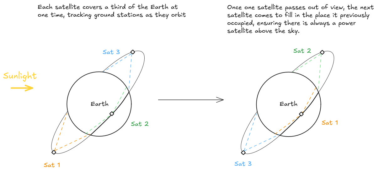
The satellite constellation ensures that there is always at least one satellite above every power station.
Let us now return to the issue of atmospheric attenuation. We have set out a feasible wavelength range of 3.75-30 cm as the suitable frequencies at which space-to-ground power transmission can realistically occur. This range can be further subdivided into four named microwave bands, from longest to shortest wavelength:
| Band name | Frequencies | Associated wavelengths |
|---|---|---|
| L-band | 1-2 GHz | 15-30 cm |
| S-band | 2-4 GHz | 7.5-15 cm |
| C-band | 4-8 GHz | 3.75-7.5 cm |
| K-band | 8-12 GHz | 2.5-3.5 cm |
In theory, using the higher end of the feasible wavelength range (that is, 15-30 cm) would lead to the minimal losses - in fact, essentially no losses. However, this runs into the unfortunate issue that as the divergence angle , these longer wavelengths cause the beam to diverge faster and become less focused, ultimately negating the advantages of their low atmospheric loss. Rather, it is a better choice to use the lower end of the feasible wavelength range (3.75 cm-7.5 cm). In fact, we will use the lowest of the wavelength range - that is, - to minimize the beam spread.
Addenum: The ITU-R model
The ITU-R atmospheric attenuation model, from the International Telecommunications Union (Radiocommunication Sector), forms the basis of the previous statement that 1-10 GHz (3.75-30 cm) microwaves can pass through the atmosphere with less than 10% loss. In the next subchapter, we will perform the relevant calculations using the ITU-R attenuation model to justify this statement. But we will take this as fact for the moment.
Determination of ideal aperture
For Project Elara, determining this ideal aperture is crucial for designing a functional laser for power transmission from orbit. The main goal we want to attain is to minimize the beam size at the power receivers (in our case, the receiver stations) on Earth, which is a formidable task considering that the beam must traverse 37,000 km from geosynchronous orbit. We may derive an expression for the beam size at the power receivers through some algebra and trigonometry.
Let the angle of divergence be the angle by which the beam diverges (spreads). Recalling that , we may write this in equivalent form as:
Over a straight-line distance along the axis of propagation, the deviation (spread) of the beam from the axis of projection would then be given by . As this is the spread from just one side of the beam, adding up the spread of both sides as well as the original beam width gives the total beam size at the receiver of . Here is a graphical diagram of the derivation we have just completed:
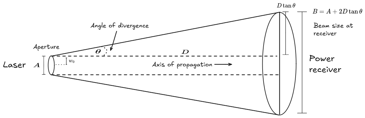
The divergence of the Gaussian beam can be approximately-modelled as circular spot that grows in radius with distance.
Given that we want a beam with minimal divergence - in fact, this would almost certainly be the most precise laser ever built - we can use the small-angle approximation as must be very small. Therefore, we have:
We want to find the value of such that the beam size at the receiver is minimized. This is a calculus-based calculation - we need to find the points at which . Taking the derivative with respect to , we have:
And setting this equal to zero, we have:
We previously discussed that we intended to use a wavelength of for optimal space-to-ground transmission, and here, is the distance to geosynchronous orbit, which is roughly 37,000 km. Thus, when evaluated, this corresponds with an ideal aperture size of approximately 1.3 km. The corresponding beam size on the ground, calculated by , is close to 2.7 km (this is the minimal beam size within our range of microwave frequencies). If we were to use the slightly shorter (and thus slightly more lossy) wavelength of , at the very edge of our wavelength range, the numbers come out to be 1.2 km for the aperture and 2.4 km for the beam size, respectively.
Now, apertures of greater than a kilometer are not as ridiculous as it would first seem, because through the technique of beam combining, smaller-aperture laser beams can be combined together into one laser beam of a much higher effective aperture. However, even with beam-combining, the substantial engineering hurdles of constructing such a laser make it non-ideal for the initial versions (though this is certainly not out of scope once we design later versions of the system).
Improved design considerations
For a more realistic design, we would want a laser with a smaller aperture, with the trade-off of some increased beam divergence. This is not simply because the optimal aperture (calculated previously), even with beam-combining, is very difficult to achieve. There is also another major issue to consider. Recall that the beam size on the ground in the optimal case is 2.4-2.7 km. As we optimized precisely for the laser to stay as collimated as possible, this also means that the 1.2-1.3 km aperture laser would need to have a 2.4-2.7 km receiver. Again, this is not impossible, and in any case the eventual design will probably be on similar scales, if not the same design. However, in this design, the receiver cannot be made any smaller, as this is already the minimal spread aperture (even if that is hard to believe!) and the laser beam is completely confined to this region, meaning that the power density within the region will be extreme. That is to say, we optimized to make an extremely efficient laser that produces a highly-focused beam; but those are exactly the properties that make the laser extremely dangerous, meaning that we must cover the entire 2.4-2.7 km diameter area on the ground with a giant receiver that can safely receive the very powerful laser beam. Understandably, this is not ideal for the initial experimental stages of the solar power satellites.
Rather, it is more feasible to construct a laser design that is purpose-built for safety. Following official regulations on microwave safety, we can design a laser that would have a relatively spread-out beam that would ensure relatively low power densities on the ground. This means that a ground receiver need not be kilometers in size; it can cover just a small area, with the portions of the beam outside of the receiver’s area passing safely into the surrounding environment. The FDA requires that household microwave ovens have a maximum power density of at 5 cm or less from the surface (21 CFR 1030.10), although this is far below a harmful dose. From some reading it appears that restaurants use up to twice that amount, at up to , which, again, is perfectly safe. If, out of an abundance of caution, we design for a power density limit of - one-tenth of the restaurant amount - then we can calculate the aperture we would need to ensure the beam was sufficiently spread-out to have this power density on the ground.
Recall that the beam size on the ground, , is the diameter of the beam by the time it reaches the Earth’s surface. Thus, we can find the cross-sectional area of the beam, which we will denote (to avoid confusion with the aperture width ), by using the typical formula for the area of a circle:
Power density (intensity) is power over area, and thus we can relate the power density limit to and the total power of the laser as follows:
Assuming the laser is ideal, the total power of the laser would be equivalent to the total power of the captured sunlight (otherwise it is less than that). If the composite solar collector is composed of hexagonal component mirrors each of side length that combine to form one paraboloid., then the total power would be given by:
Where is the mean solar irradiance (the average intensity of sunlight at Earth orbit). To solve for the aperture width that would satisfy our power density limit, we can substitute in the expression for into the expression for , resulting in a quadratic equation:
We may solve the quadratic equation by applying the quadratic formula, and thus we have (after some simplifying):
This, however, requires that to get a sensible answer for . Thus the minimum total power required for a real solution is given by:
Which calculates to , approximately equivalent to the total power collected by a 115m radius flat (circular) mirror. This is also around equal to a composite mirror composed of 500 hexagonal segments each with 5.5m sides (although this is also an approximation because this also presumes a flat, not parabolic, shape). This means that for all the mean power density on the ground is within the safe limit (which, again, is a very conservative limit). The larger we make the composite mirror in space (by adding more hexagonal segments), the smaller the aperture can be to guarantee the same safe power density while also increasing the total power received on the ground, so it is advantageous to make the composite mirror as big as possible. The following table (calculation spreadsheet available at this link) showcases values for the number of hexagonal mirrors needed and aperture width required:
| Effective aperture width | hexagonal mirrors required | hexagonal mirrors required | hexagonal mirrors required |
|---|---|---|---|
| 1.329 km | 157 | 519 | 1744 |
| 313.77 m | 785 | 2594 | 8720 |
| 215.69 m | 1570 | 5190 | 17440 |
| 174.55 m | 2355 | 7784 | 26160 |
| 122.36 m | 4709 | 15567 | 52320 |
| 94.46 m | 7848 | 25944 | 87199 |
| 66.62 m | 15696 | 51887 | 174398 |
These aperture values are effective aperture values (i.e. aperture after beam combining), so the actual apertures of the individual lasers do not have to be this large. As a general approximation, an effective aperture of can be achieved with individual lasers of aperture by . By rearrangement, we can solve for with:
The below table lists the number of individual lasers required to attain the effective aperture for individual lasers of different apertures:
| Effective aperture width | Number of aperture lasers required | Number of aperture lasers required | Number of aperture lasers required | Number of aperture lasers required | Number of aperture lasers required |
|---|---|---|---|---|---|
| 1.329 km | 873 | 2826 | 17663 | 70650 | 196249 |
| 313.77 m | 49 | 158 | 985 | 3939 | 10940 |
| 215.69 m | 23 | 75 | 466 | 1861 | 5170 |
| 174.55 m | 16 | 49 | 305 | 1219 | 3836 |
| 122.36 m | 8 | 24 | 150 | 599 | 1664 |
| 94.46 m | 5 | 15 | 90 | 357 | 992 |
| 66.62 m | 3 | 8 | 45 | 178 | 494 |
The numbers, certainly, are formidable, but they are not out of reach. The hexagonal mirrors can be launched in batches, slowly, over the course of decades, with the solar power satellite providing more and more power over time, until it reaches full power. While the mirror numbers may seem staggering, remember that these mirrors are in space and therefore need no active support, and they can be made extremely thin and lightweight; their only requirement is to be reflective. Additionally, they can be folded to a very small size, then expand once they reach orbit, meaning that with some creative folding they can be made to take up relatively little room aboard a rocket. The much bigger engineering challenge, at least on paper, are the individual lasers, considering their very large apertures, even just individually.
A constructible prototype design
It is important to note that so far, we have been discussing only designs on the very large-scale. However, our first space launch is likely to be a far, far smaller design - most likely a satellite on the order of a few thousand kilograms, deployed into orbit over three launches. Some rough reference parameters are listed below:
| Power satellite mass | Power satellite orbit | Satellites in constellation | Mirror mass | Total payload size |
|---|---|---|---|---|
| ~5,500 kg | Geosynchrnous | 3 | ~500 kg | ~6000 kg |
The composite solar mirror would “ride along” with the power satellites and be launched alongside, in a folded compact configuration, until both reach orbit, at which point the mirror segments unfurl and lock together. Each segment would be hexagonal and very thin. Again, some reference parameters are listed below:
| Composite mirror segments | Segment side length | Fully-unfurned diameter | Total captured power |
|---|---|---|---|
| 5-55 segments | 3-5m | 20-40 m | 428 kW - 1710 kW |
Each power satellite is anticipated to have a large number of small lasers, using beam-combining to achieve a greater effective aperture. We must unfortunately use shorter wavelengths as the much smaller effective apertures as compared to the designs we previously examined mean that the lasers diverge far more quickly, even though we know that longer wavelengths are better at passing through the atmosphere without being affected by weather conditions. Below are some rough values for the projected power beam laser[1]:
| Feed laser aperture | Wavelength | Number of beam-combined feed lasers | Effective aperture | Ground beam width | Ground power density | Received power |
|---|---|---|---|---|---|---|
| At least 25 cm | 1-2 cm | At least 200 | >350 cm | 133-266 km | to | 0.6 - 9.6 mW |
On Earth, the receiver would also be rather small compared with our previous designs - we envision a 10-meter (diameter) receiver parabolic antenna, which is used to calculate the received power in the last column. In addition, the receiver antenna will not be a custom one; it will likely involve a temporary (or permanent) lease of a pre-existing telecommunications antenna. Of course, the larger the receiver, the better; however, the received power is likely to be rather weak, about 8 times as powerful as a household AA battery in theory, but perhaps only half as powerful in reality. Even in the best possible case (such as, for instance, if we hypothetically used NASA’s 70m Deep Space Network antenna as the receiver), the received power would still be under half a watt, or at most, a few watts.
So it should be emphasized that this is a research testbed to test out the system design in a real-world environment, which must be undertaken before building any large-scale solar power satellites for practical energy generation. This means that we don’t expect this testbed to actually produce any useful amount of energy[2], and while the mirrors will be re-used (recall that the hexagonal mirrors can be continuously extended with more segments), and the receiver antenna returned to its operator, the power satellite will be placed in a graveyard orbit after its useful lifetime. In some sense, it would be like a Chicago Pile for Project Elara’s solar power satellites - essentially, a proof-of-concept.
The received power values are assuming a 10-meter (diameter) ideal receiver antenna. In addition, the ground power density values are not accounting for atmospheric attenuation, which, at such short wavelengths, can mean losses up to 50% or more in heavy rain or stormy weather, even if losses are within 10% during clear skies.
Do note, however, that commercial satellites have even weaker signals, so weak that even the milliwatt power levels in the projected testbed are orders of magnitude more powerful than nearly all satellites in similar orbits.